Overview
PyLag is an offline particle tracking model. The model expects as inputs time independent and/or dependent variables that describe the state of a given fluid. These may be measured quantities or the predictions of an analytical or numerical model. Using these, the model computes Lagrangian trajectories for particles released into the fluid at a particular point in time and space. The model is primarily aimed at marine applications, but in principle could be extended for use in other contexts too; for example, in studies of atmospheric dispersion.
PyLag was created with the aim to make available a particle tracking model that is a) fast to run, b) easy to use, c) extensible and d) flexible. The model is written in a mixture of Python and Cython. Here we provide a brief overview of the code structure, and some of the model’s key features.
Code structure
A simplified Unified Modelling Language (UML) Class Diagram for the model is shown in Figure 1. Functions that perform numerically intensive tasks have been implemented in Cython or C++ (dark grey boxes), while those that perform less numerically intensive tasks have been implemented in Python (pale grey boxes). The division is intended to combine the ease of use of Python with the efficiency gains offered by Cython and C++. During compilation, Cython source files are parsed and translated into optimized C++ code, which is them compiled into extension modules that can be loaded at runtime by the Python Interpreter.
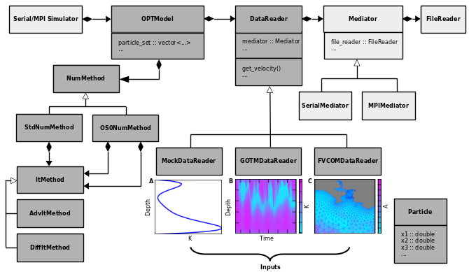 Figure 1 UML Class Diagram.
The model currently includes direct support for the General Ocean Turbulence Model (GOTM), the Finite Volume Community Ocean Model (FVCOM), the Regional Ocean Modellling System (ROMS) and data defined on a regular Arakawa A-grid, as is typical of datasets downloaded from public catalogues (e.g. the CMEMS). Further details on the types of input PyLag accepts are given below. To simplify the diagram, only GOTM and FVCOM are depicted in Figure 1.
Each input source has associated with it a derived DataReader class that inherits from a base class DataReader (see Figure 1). The primary purpose of such objects is to compute and provide access to the value of a given variable (e.g. the vertical turbulent eddy diffusivity) at a particular point in space and time. For gridded input data, this process is facilitated through interpolation, while taking into account the structure of the underlying model grid. Figures 1B and 1C give
examples of the types of input generated by GOTM and FVCOM respectively: the former shows a Hovemoller diagram of the simulated vertical turbulent eddy diffusivity for heat at a location in the Western English Channel; the latter a map of the surface horizontal turbulent eddy diffusivity field near to the coastal city of Plymouth, UK. The code has been designed in a way that makes it possible to easily extend the model to read in data defined on different types of input grid. This can be
achieved by sub-classing DataReader.
When working with 2-D or 3-D data, PyLag creates an unstructured horiztonal grid or grids to assist with locating particles and interpolating input data to particle positions. This occurs irrespective of the type of grid on which the input data is defined. When working with FVCOM, which uses an unstructured grid, PyLag simply adopts FVCOM’s grid directly, after ensuring all information regarding neighbouring elements is ordered as PyLag expects. When working with data defined on a regular Arakawa A-grid, PyLag first creates an unstructured representation of the grid. In all cases, the required information is encoded within a dedicated grid metrics file which PyLag reads at the start of the simulation.
Given input data, PyLag can compute particle trajectories using one of the different numerical schemes implemented in the model code. In order to support numerical methods that employ some form of operator splitting in which advection and diffusion are handled separately, two different families of object have been implemented. Objects that belong to the first family control the integration process, and may or may not implement some form of operator splitting. They inherit their interface from
the base class NumMethod. Two derived classes have been implemented: StdNumMethod and OSONumMethod. The former does not employ operator splitting, while the latter implements a basic form of operator splitting. Objects from the second family represent iterative methods that have no awareness of whether operator splitting is being used: they simply compute position deltas, and return these to the caller. They inherit their interface from the base class ItMethod. Several derived
classes have been implemented: some of these implement pure deterministic solution methods that should be used for advection-only problems; others implement purely stochastic solution methods that should be used for diffusion-only problems; while others implement solution methods that are suitable for problems involving both diffusion and advection.
The testing of such models is facilitated through the inclusion of various mock classes that are derived from DataReader. Mock classes typically encode analytic functions that describe the spatio-temporal variability of a given field variable or variables (e.g. the velocity field). This removes the dependency on external input data. Figure 1A shows an example of a vertical turbulent eddy diffusivity profile computed using an analytic formula. The same profile is used in one of PyLag’s
examples to test for the Well Mixed Condition.
Wave and atmosphere coupling
Support was using PyLag with atmosphere and wave data, and modelling the influence of windage and Stoke’s Drift on particle transport dynamics, has been included in the PyLag softward package. Figure 2 shows a UML Class Diagram, which illustrates how PyLag handles multiple sources of input data. This is achieved using an adaptation of the Composite Design Pattern, and the inclusion of a CompositeDataReader class which includes separate data readers for ocean, wave and atmospheric data. These data readers work just like the ocean data readers, with their own grid metrics file which contains information regarding the grid layout.
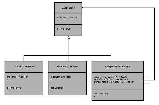
Figure 2 UML Class Diagram showing how multiple data sources can be used together.
A degree of flexibility in how the wave and atmosphere data is used is facilitated through the inclusions of a family of objects which inherit from the base classes StokesDriftCalculator and WindageCalculator respectively. An object of type VelocityAggregator, which holds a reference to the selected Stoke’s Drift and Windage calculators, is used to pool and combine the impact of these different processes on a particle’s velocity vector.
An end to end example of running PyLag with Stoke’s Drift and Windage can be found here.
Supported models and grid types
A summary of the hydroynamic models and sources of input data supported by PyLag is given in Table 1. PyLag was initially developed to work with input data generated by FVCOM. It was then extended to work with input data generated by GOTM and ROMS; and data formats that are common to public ocean data repositories, such as the CMEMS catalogue.
Typically, data made publicly available through large repositories, such as the CMEMS catalogue, is formatted to meet community standards which were introduced to facilitate intermodel comparison studies. Typically, the data are provided on a regular latitude-longitude grid with fixed depth levels. If the model used to generate the data employed a different type of grid, the data is first post-processed before being made publicly available. In the post-processing step, scalar and vector quantities are interpolated onto a common grid, and velocity vectors rotated as required. The final grid format is consistent with the Arakawa A-grid type, in which all variables are defined at cell centres. The grid is typically regular, with latitude and longitude coordinates given by 1D arrays. With PyLag, curvilinear grids are also accepted; however, there is a restriction that the \(u\) and \(v\) velocity components should be alligned with East and North respectively. If this is not the case, the velocity components should be rotated before being passed to PyLag. Lastly, it is common that variable names adhere to Climate Model Output Rewriter (CMOR) standard names. However, this is not a requirement for PyLag.
As support for new models is added to PyLag, Table 1 will be updated. Examples of running PyLag with the existing set of models can be found here.
Table 1 Hydrodynamic models and data catalogues with fixed format specifications that are supported PyLag.
Source |
Description |
Spatial dimensions |
Horizontal grid type |
Horizontal coordinates |
Comment |
|---|---|---|---|---|---|
GOTM is a one-dimensional,
relocatable water column model
that includes state-of-the-art
descriptions of vertical
mixing (Umlauf et al 2008).
|
1D
|
N/A
|
N/A
|
||
FVCOM is a prognostic,
unstructured-grid, finite-volume,
free-surface, 3D primitive equation
coastal ocean circulation model
(Chen et al 2003).
|
3D (local or
regional scale)
|
Unstructured triangular
mesh.
|
Geographic and Cartesian
|
||
ROMS is a free-surface,
terrain-following, primitive
equations ocean model widely used
by the scientific community
for a diverse range of applications
(e.g., Haidvogel et al., 2000).
|
3D (local or
regional scale)
|
Arakawa C-grid (rectilinear
and curvilinear)
|
Geographic
|
||
CMEMS public catalogue for
near real time and reanalysis
products. Entry covers products
provided on a standard Arakawa A-
grid and adhering to community
standards.
|
2D and 3D (local,
regional or global
scale)
|
Arakawa A-grid (rectilinear
and curvilinear)
|
Geographic
|
u and v velocity components
should be alligned with true
east and north respectively.
|
Serial and parallel execution
The particle tracking model lends itself to parallelization since the particle set can be readily broken up and scattered over multiple processors that independently compute changes in state for each particle they manage. This approach has been applied using MPI for Python. A Mediator class (Figure 1) facilitates the switching between serial and parallel execution without the need to either recompile the code or unnecessarily set operating system environmental variables.
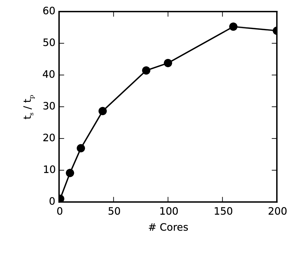
Figure 3 MPI scaling.
Short duration benchmark runs using a seed of \(10^6\) particles show that, when compared with serial execution, this can reduce run times by a factor of 50 or more; however, for large numbers of processors (100s or more), gains can become limited by broadcast and gather operations, as well as the time needed to import shared libraries (Figure 2). Ultimately, the performance of MPI runs will depend on the run being performed. Generally, performance will be greatest in longer runs involving many particles, and in which read/write operations are performed relatively infrequently.
References
Chen, C. H. Liu, R. C. Beardsley, 2003. An unstructured, finite-volume, three-dimensio nal, primitive equation ocean model: application to coastal ocean and estuaries.J. Atm. &Oceanic Tech., 20, 159-186
Haidvogel, D. B., H. G. Arango, K. Hedstrom, A. Beckmann, P. Malanotte-Rizzoli, and A. F. Shchepetkin (2000), Model evaluation experiments in the North Atlantic Basin: Simulations in nonlinear terrain-following coordinates, Dyn. Atmos. Oceans, 32, 239-281.
Umlauf, L. Burchard, H., 2004. Second-order turbulence closure models for geophysical boundary layers. A review of recent work. Continental Shelf Research 25(7):795-827. DOI: 10.1016/j.csr.2004.08.004|